Guitar Amp Simulation with Tensorflow and Keras
I design and build vacuum circuits for a hobby, and I also play electric guitar, so it was only natural that I build myself a guitar amp. Tubes are prized by guitarists for their tone when driven into clipping – it’s no exaggeration to say that the sound of rock and roll guitar is the sounds of tubes being driven into overdrive.
Early instrument amplifiers were not designed to produce distortion, but guitarists turned them all the way up to get distorted tones from the power tubes. Later, amp builders added specifically-tuned circuitry in the preamp section, so guitarists could get distorted tone without having to saturate the power tubes. Modern high-gain amp designs have cascading gain stages, each of which can generate clipping, with various tone-shaping elements between stages to affect the frequencies at which clipping occurs. Different designs by different manufacturers have dedicated followings among guitarists.
Lately, there have been devices on the market that mimic the sound of tube amps using digital signal processing (“DSP”). I’m no expert on DSP, but I tried the Line 6 POD when it came out, but I haven’t tried the more recent Axe-fx by Fractal Audio Systems that is very popular these days.
I started wondering: deep learning shows promise in part because the early layers can learn their own representations of the data, rather than having humans do a lot of pre-processing and feature engineering -- convolutional neural nets trained on images of faces, for example, will automatically learn features that correspond to eyes, noses, mouths, and so on. Could deep neural nets do a good job learning the function that takes a clean guitar signal and produces a good-sounding distorted tone?
The Input Data
I recorded a stereo track of my electric guitar – the left channel is a direct recording of the signal straight from the guitar, while the right channel is the sound of the amplifier as recorded by a microphone. The microphone is the industry-standard SM57, and it was positioned about one inch from the speaker grille, pointed right at the cone. I would have liked to crank up the amplifier to get a good mix of preamp and power amp distortion, but I had to settle for only preamp distortion, because I live in an apartment. Here’s the audio of the training data (note that these samples have been converted to MP3 to put on the web – the actual files used were large, uncompressed data at 44.1kHz, 16 bit). I tried to get a good mix of quiet and loud signal coming from the guitar.
Right away, we are throwing a big challenge at our algorithm. We expect our neural net to learn not only the distortion characteristics of the electronic amplifier, but also all contributions to the sound caused by nonlinearities in the speaker cone, the microphone, the echo of the room, and even the air itself.
So far, so good. Let’s load this data into an iPython notebook and see what we can see:
%pylab inline
import numpy as np
import pandas as pd
import seaborn, matplotlib
seaborn.set_style('whitegrid')
from copy import deepcopy
import pickle
import wave
import time
import soundfile as sf
matplotlib.rcParams['xtick.labelsize'] = 14
matplotlib.rcParams['ytick.labelsize'] = 14
matplotlib.rcParams['axes.labelsize'] = 14
matplotlib.rcParams['axes.titlesize'] = 16
matplotlib.rcParams['figure.titlesize'] = 16
matplotlib.rcParams['legend.fontsize'] = 16
matplotlib.rcParams['figure.figsize'] = (10, 5)
data, samplerate = sf.read('GuitarTraining.wav')
direct = data[:,0]
amp = data[:,1]
We will use the package soundfile to convert our stereo WAV file into two one-dimensional numpy arrays, one array for each stereo channel. Ok, let’s plot the data:

This looks about like we would think. The direct signal has much more dynamic range, whereas the recorded amplifier signal is “squashed” because the amp clips the waveform by purposefully driving the triodes beyond their linear range. When playing with distortion, picking the strings softer doesn’t result in a quieter sound from the amp, but rather a less distorted sound.
Let’s zoom in:
plot_start = 800000
end_window = 1000
amp_plot = amp[plot_start: plot_start + end_window]
direct_plot = direct[plot_start: plot_start + end_window]
plt.plot(amp_plot + 0.5, label = 'amp')
plt.plot(direct_plot, label = 'direct')
plt.title('Waveforms Closeup')
plt.legend()

Now this looks interesting! The amp signal doesn’t look simply like a “clipped” version of the clean tone. Whatever function is transforming the direct signal into the mic’d signal looks pretty complicated. To the eye, the clean waveform looks sort of truncated in places, but with a higher-frequency signal superimposed on it. This also makes sense, ultimately: the design of the amplifier doesn’t simply boost and then clip the signal. Rather, clipping happens in stages, and there are EQ adjustments at almost every step (for example the cathode bypass resistors of the gain stages are rather small so that low-frequency response is limited). This is part of what makes one guitar amp sound different from another.
Design of the Neural Net
So, with our data selected, how will we design our algorithm? Let’s take a step back and consider what we’re trying to do. Our input is a one-dimensional array of values between -1 and 1, with a length equal to 44,100 * length of the recording in seconds. Our output will also be a one-dimensional array within the same range of values, and should be about the same length (if we lose some data because we have a window, that’s ok). So, we want our algorithm to learn a function that converts an input vector into an output vector. We won’t worry about real-time signal processing for now, and given that neural nets are so computation-heavy, this will probably remain a secondary concern.
But let’s take this a little further. How long should the input vector be? Ideally, we want to be able to convert a recording of a clean guitar at any length to the proper output. Thus, we shouldn’t rely on pre-defining the length of the input vector. With that in mind, let’s ask ourselves – what portion of the input signal at time t do we expect to have an effect on the output signal at time t? This will tell us how to structure the data we feed into the algorithm. Obviously, anything that the guitar does in the future can’t affect what the amp does now. But how far in the past should we let the algorithm look?
This is not a trivial question. A totally straightforward clipping algorithm would not need any history at all – it would simply have a floor and ceiling of the waveform, and if the instantaneous value of the input signal exceeded those, the algorithm would simply return the value directly within the floor or ceiling until the wave fell back within the defined limits. We know from visualizing the waveform above that the amp isn’t doing anything this simple.
In addition, we should take into account what we know about how amplifiers work. There are various ways in which an amp’s instantaneous state would be dependent on the path it took to reach that state. For instance, the speaker has some elasticity and would store energy from its previous trajectory. The power supply is non-linear, and would be expected to “sag” somewhat after a large impulse (especially since this amp uses a tube rectifier). Even the iron core of the output transformer has hysteresis loss from the fluctuating current. The fact that we have a microphone recording a speaker cone in a room makes things even worse: the signal at the microphone’s diaphragm would contain at least some sound that has been bouncing around the room for some appreciable fraction of a second. Again, we are asking a lot of our algorithm.
Calculating the time frame for all these effects would be beyond the scope of this little experiment, so I decided to simply assume that the signal presented to the amp in the last 1/10th of a second would be fed into the algorithm. This window would theoretically allow frequencies down to 10Hz to be detected, and this is far below any frequencies generated by a guitar. I would “cheat” and allow the algorithm to see a small number of points into the future, to account for any latency/lag in the signal coming from the amp (this was probably not useful, but it shouldn’t hurt either).
So, now we know that for every moment (44,100 moments per second), we want the neural net to produce one float value representing the value of the recorded amp. The input will be 4000 points mostly preceding that moment.
def make_xy(direct, amp, start_ind = 0, end_ind = 10000, window = 600, future = 10):
if not end_ind + future < len(direct):
print('ERROR: Indices extend beyond data')
return 0
if not len(direct) == len(amp):
print('ERROR: direct signal and amp signal must be of equal lengths')
return 0
time1 = time.time()
start_ind = max(start_ind, window)
list_X = []
list_Y = []
for k in range(start_ind, end_ind):
list_X.append(direct[(k - window + future) : k + future ])
list_Y.append(amp[k])
X_arr = (np.array(list_X, dtype = 'float32'))
Y_arr = np.array(list_Y, dtype = 'float32')
time2 = time.time()
print('Time to make XY: {0:.2f}'.format(time2 - time1))
return X_arr, Y_arr
window = 4000
future = 300
X, Y = make_xy(direct, amp, start_ind = 250000, end_ind = 800000, window = window, future = future)
X_test, Y_test = make_xy(direct, amp, start_ind = 800000, end_ind = 1500000, window = window, future = future)
[EDIT: with the newer version of Keras, I would certainly use TimeseriesGenerator instead of making this array in memory.]
Now that we have our training data (about 12 seconds of guitar playing from the beginning of the recording), let’s define and build the neural net:
from keras.models import Sequential, Model
from keras.layers import Dense, Dropout, Activation, Input
from keras.utils import np_utils
from keras import backend as K
K.set_image_dim_ordering('th')
model = None
model = Sequential()
model.add(Dense(256, activation = 'relu', input_shape=(window,)))
model.add(Dropout(0.5))
model.add(Dense(256, activation = 'relu'))
model.add(Dropout(0.5))
model.add(Dense(256, activation = 'relu'))
model.add(Dropout(0.5))
model.add(Dense(1, activation = 'tanh'))
model.compile(loss = 'mean_squared_error',
optimizer = 'RMSprop',
metrics = ['accuracy']
)
history = model.fit(X, Y,
batch_size = 256, epochs = 2, verbose =1)
Our neural net will have dense layers – every input value will be connected to every neuron in the next layer. Why not use convolutions? Well, we are dealing with a continuously variable input vector that can have any frequency (because we might play any note of the guitar), so we have no reason to expect that there will be some reasonable number of identifiable “motifs” that will provide us with useful information, the way that all frontal photographs of cat faces look sort of the same. Why not something like an LSTM, which is commonly used to model time series data? Answer: we are not trying to predict the future of the amplifier signal based on the past of the amplifier signal – rather, we are trying to learn the function that transforms the clean signal into the amp’s distorted signal, and we are even willing to look into the future of the training data a little. This is a regression problem.
There is nothing magical about using three layers of 256 nodes each, or the proportion of dropout – these were chosen as reasonable prior parameters. The choice of tanh for the output is dictated by the data – the output signal varies between -1 and 1, so this is a natural choice of activation function. Mean squared error is a natural choice for what is basically a regression problem. Let’s train the model:
Epoch 1/2
550000/550000 [==============================] - 6s - loss: 0.0025 - acc: 2.8909e-04
Epoch 2/2
550000/550000 [==============================] - 6s - loss: 0.0015 - acc: 2.8909e-04
Training took just a few seconds on my computer. Hrm, this seems reasonable enough, but how does it sound? To see, we will use our test data, which the model has never seen. We’ll make predictions and compare with the real amplified signal. First, here is the real amplifier:
Here is the output of the model on the same signal:
To the ear, the results don’t sound terrible, but not quite like the real thing either. To me, the model output has a different midrange character, less like a mic’d amp and more like a Fuzz Face pedal plugged directly into the mixing board. The real sample also sounds distorted, but also has an identifiably Marshall-like focus in the midrange.
Further tests involved more or less the same model with different numbers of layers (one and two hidden layers), and different optimizers. Overall, the subjective quality of the output was more or less the same most of the time (the model with one hidden layer seemed to produce less “fizz” in the high frequencies). One interesting result was obtained with two hidden layers and SGD as the optimizer. This model obtained a lower training loss score of 0.0084, but the test sample sounded like the volume was fluctuating rapidly:
This is probably caused by overfitting, but the volume effects are a strange artifact (possible due to the microphone picking up ambient sound from the room?) I did not use cross-validation during training, because the models converged very quickly, and evaluation on the cross-validation set only happens at the end of every epoch, limiting its usefulness in conveying information about the training.
Discussion
As a first, quick-and-dirty attempt, the neural net amp simulator is a qualified success. The output on test data at least sounds like a distorted guitar with most models, so it seems our model is at least learning some kind of distortion function on the input waveform. Further refinements should take several factors into account.
First, matching a waveform may not be the best way to train a guitar amp simulator that sounds good to the ear. The human ear is much more sensitive to midrange frequencies than to highs and lows (this is the range of human speech, the analysis of which is very important from an evolutionary standpoint). Thus, accurately modeling the subtleties of the midrange of a guitar amp is much more important than getting the lows and highs correct – but the simple mean squared error on a waveform does not capture this important aspect of a good amp model. Furthermore, the human auditory system cannot hear phase relationships between frequencies, provided that the phase differences are not shifting. Thus, humans cannot tell the difference between 1) a 1000Hz triangular wave; and 2) a wave that has all the same harmonics as a triangular wave at the same amplitudes, but each harmonic shifted so that the overall wave no longer looks triangular. This suggests that matching a precise waveform may not be the most important thing to get right for our model.
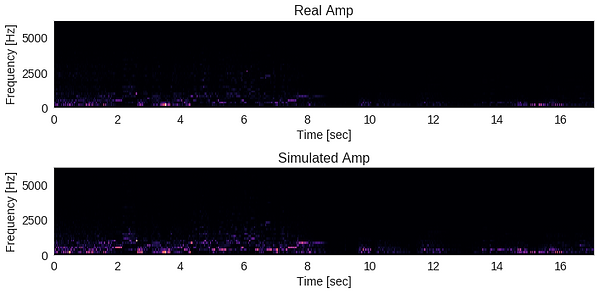
Secondly (and related to the first point), it may be helpful to provide engineered frequency information to the input of the neural net, and somehow add frequency accuracy to the loss function that the model is trying to minimize. As it is, the neural net has no direct understanding of frequency at all, other than what it can learn from the raw waveform. This seems a lot to ask, even for a deep neural net. Some kind of feature engineering, possible involving the fast Fourier transform, may provide the neural net with more useful information. A quick visualization shows that the frequencies of the real and simulated guitar amps are different:
Hopefully, future attempts conducted with these considerations in mind will yield a better-sounding amp simulator. If you would like to tackle this project and would like the original training set file in uncompressed audio, please contact me.